Thermal processes · Technical article
Thermal Matching in open combustion engines
Qualifying and quantifying the high-temperature interaction in Brayton, Diesel and Otto engines.
Summary
A closed-cycle heater receives heat through an identifiable external interface. In a direct-fired engine, fuel and oxidiser react within an evolving gas mixture. The latter can still be examined with temperature-resolved local balances: an externally adiabatic combustor may contain real internal heat conduction across finite gradients. This article connects that established transport physics to an explicitly qualified Thermal Matching interpretation, with a calculated two-volume example and the A1 thermal-network animation. It does not equate chemical reaction with external heat input, or infer engine efficiency from a temperature diagram alone.
At a glance
- Established: internal conductive transfer and its entropy generation can be resolved under a specified model.
- Proposed: an ETS–TM donor–receiver reading may organize selected physical transfers for Thermal Matching.
- Illustrative: the two-volume calculation and 49-node animation do not resolve reacting-flow chemistry or engine work.
1. The comparison with a closed heat engine
For an externally heated closed heat engine, a high-temperature source and a working medium are identifiable on either side of a physical interface. Their local temperatures and heat increment can be paired along a T–Q trajectory. A finite temperature gap makes that particular thermal contact irreversible. The complete engine also has a low-temperature interaction and a work balance.
In a direct-fired engine, chemical energy enters with fuel and the reaction takes place inside the working flow. There is no automatically corresponding external hot stream or wall carrying the modelled high-temperature heat input. The useful comparison is therefore between specified physical interactions and complete balances, not between visually similar curves alone. A local donor–receiver representation can be considered only after its actual transport mechanism is identified.
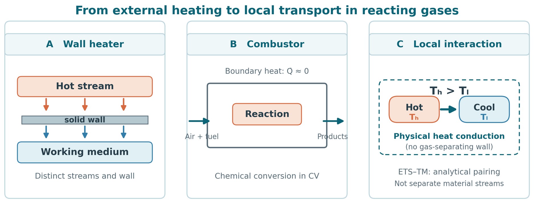
| Question | Externally heated closed cycle | Direct-fired open engine |
|---|---|---|
| High-temperature energy input | Heat crossing a specified interface from an external source. | Fuel and oxidiser enter as material streams; reaction changes the mixture’s chemical and thermal states. |
| Physical thermal transfer | Heat flux through the heater wall and adjacent boundary layers. | Selected internal conduction, radiation or other transport across defined local faces; wall loss if the outer boundary is non-adiabatic. |
| Quantification | Paired stream temperatures, heat duty, conductance and entropy balance. | Resolved temperature, species and flow fields; non-overlapping local transport and reaction terms, then a complete component and cycle balance. |
2. An adiabatic boundary and internal transport
“Adiabatic combustor” describes a chosen outer control-volume boundary: external heat transfer through that boundary is approximately zero. It does not mean that the interior is isothermal. A reacting region may be hotter than adjacent gas; molecular conduction can carry energy across their shared internal face. Those internal face transfers cancel algebraically when the adjacent energy balances are added, but their entropy production does not cancel.
At a continuum scale where local equilibrium and isotropic Fourier conduction apply, the conductive heat flux and its local entropy-generation rate per volume are:
Fourier conduction and its entropy production
The temperatures are absolute; k is thermal conductivity. This term accounts for conduction. Reaction, species diffusion, viscous dissipation and other mechanisms require their own consistent terms in the full entropy balance [2].
3. Brayton, Diesel and Otto: cycle model versus combustion
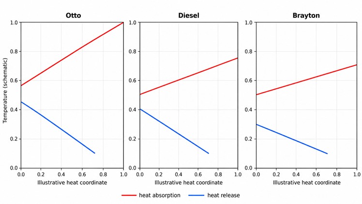
Idealised, calorically perfect air-standard cycle models use a rising heat-addition trajectory:
Specific heat addition in ideal cycle models
With constant heat capacity, T rises linearly with cumulative model heat addition. The q-coordinate is a cycle-model surrogate. It does not measure heat crossing the outer casing of an actual combustor, nor does it map a flame’s location.
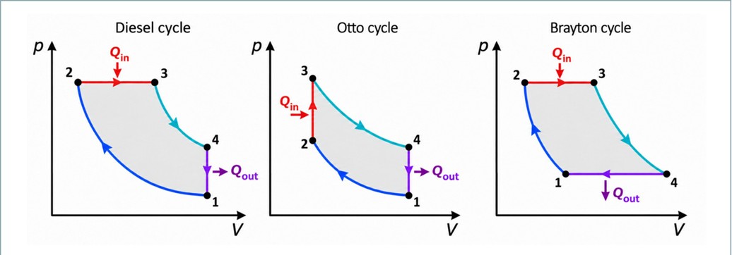
| Engine | Idealised heat-addition branch | Actual process to resolve | Suitable boundary and time description |
|---|---|---|---|
| Open Brayton | Approximately constant pressure; q follows cpΔT in the air-standard model. | Continuous reacting throughflow, injection, recirculation, dilution and pressure loss. | Stationary combustor control volume plus local spatial fields; transient fields where needed. |
| Diesel | Constant-pressure heat addition in the ideal cycle. | Injection, evaporation, autoignition, mixing and reaction during a changing cylinder volume. | Crank-angle or time-resolved moving cylinder and local reacting regions. |
| Otto | Constant-volume heat addition in the ideal cycle. | Spark initiation, flame propagation and interactions between burned and unburned gas. | Crank-angle or time-resolved moving cylinder, with appropriate local zones. |
The three models share a non-isothermal cycle-level branch under these assumptions; their real combustion fields and comparison constraints differ. Even an approximately constant-pressure gas-turbine burner has pressure loss and a fuel-dependent outlet state [3].
4. A changing mixture, not two permanent streams
The physical starting point is one spatially non-uniform reacting mixture. A small region may contain fuel, oxidiser, intermediates and products while its temperature and composition change. Chemical conversion can raise its sensible energy; conduction can redistribute energy to a cooler neighbour; species diffusion, advection, radiation and pressure work may occur at the same time. These are simultaneous terms of a local balance, not successive, isolated devices.
A finite-volume grid is an analytical partition of this field. A cell face is a specified surface for flux accounting; it does not make adjacent cells sealed reservoirs. A stationary cell may receive different material as flow proceeds, whereas tracking a moving gas parcel calls for different advective bookkeeping. In an Otto flame, burned and unburned zones can be useful descriptive regions, but neither is a permanently separated heat-exchanger stream.
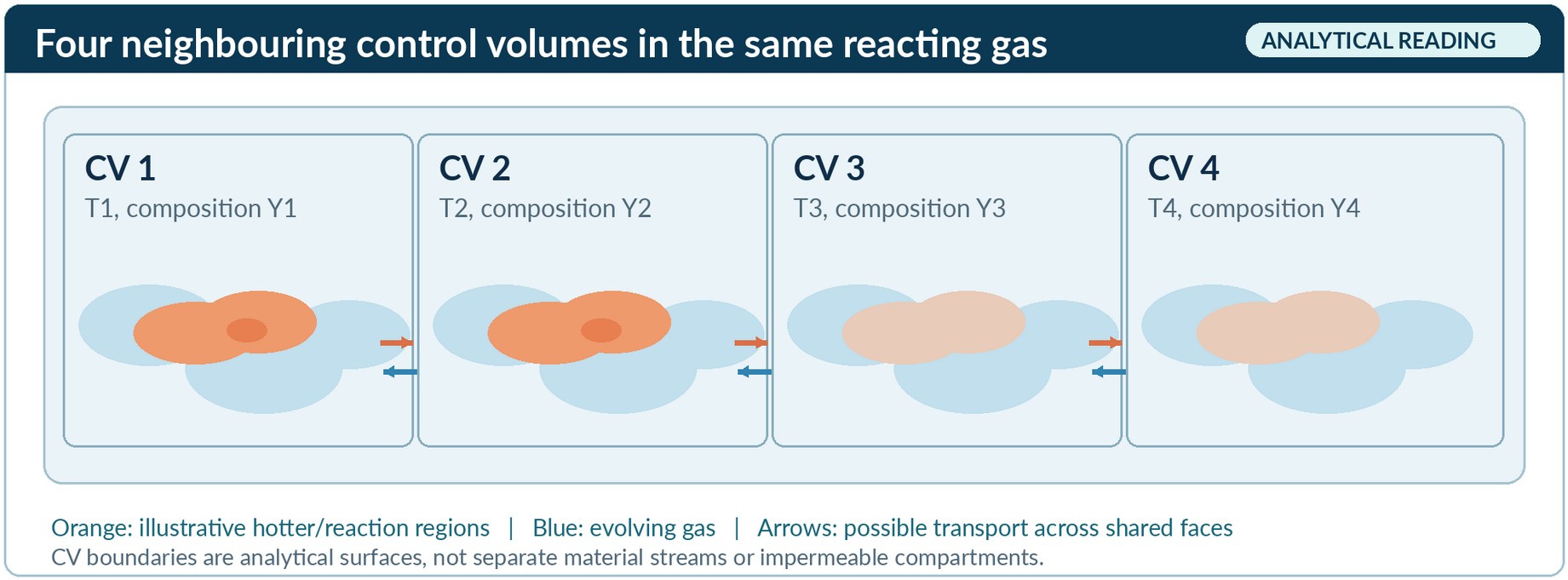
Consequently, fuel-vapour fraction cannot be read as the geometric fraction occupied by a hot or reacting zone. Such a zone needs an operational criterion, such as a reaction-rate or progress-variable threshold, and sensitivity checks for grid size, averaging interval and threshold. The temperature gradient, actual transport coefficients and specified face determine a conductive flux; an assigned ETS–TM temperature gap does not [1].
5. What can be quantified locally?
A physically attributable local analysis begins by choosing a control volume, observation interval and transfer mechanism. Temperature and composition fields determine properties; a resolved internal face supplies a heat flux and direction. For a face normal pointing from donor i to receiver j, the selected conductive transfer is:
Conductive energy through a specified internal face
Species enthalpy transport, advection, radiation and chemical conversion are recorded separately. Integrating σcond over the chosen volume and time gives its conduction-related entropy generation. For a declared reference environment T₀, the corresponding destroyed exergy contribution, if the decomposition is consistent, is:
Exergy destruction attributed to conduction
The total combustor exergy destruction requires the total entropy generation, including reaction and other transport mechanisms. Exergy destruction is a work-potential measure relative to T₀, not missing energy or an independently recoverable shaft-work output.
This makes open and closed arrangements comparable at the level of declared energy, entropy and exergy accounts. It does not make their high-temperature mechanisms identical. A temperature gap constructed between analytical labels is insufficient to calculate a flux or loss.
6. A bounded two-volume calculation
Take two neighbouring idealised gas volumes inside an externally adiabatic boundary. For one short interval, region A is at 1600 K and region B at 1000 K. Suppose 100 J is conducted from A to B and their temperatures can be treated as approximately constant during the increment. Then the heat lost by A equals the heat received by B.
Illustrative conduction entropy generation
Destroyed exergy for T₀ = 298 K
These are indicative calculations for one isolated internal conductive interaction [1]. They are neither a measured combustor result nor its total irreversibility. Any simultaneous chemical reaction in A changes the species and energy account there; it is not a second conductive flux across the A–B interface. Actual fields, interface area and interval would have to be determined by measurement or a validated reacting-flow model.
7. Animation: repeated heating in a 49-node network
The copied A1 animation extends the two-volume calculation to a 7 × 7 network of 49 finite thermal nodes. Each node has a prescribed sensible-energy capacity and conducts energy to its nearest neighbours. Three localized energy pulses are imposed in succession. A white outline follows one receiving node as it warms, exchanges energy with neighbours and may be warmed again. The graph in the video shows its temperature history alongside selected source-node histories [1].
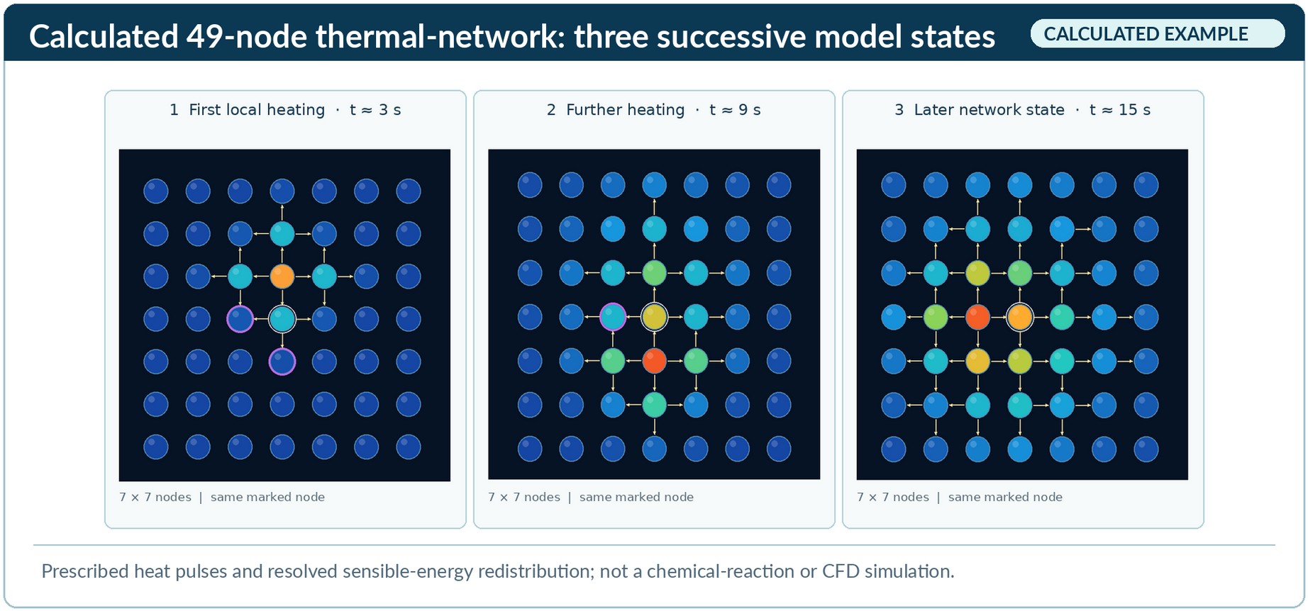
Supplementary Animation S1 · Model A17 × 7 thermal network · three prescribed pulses
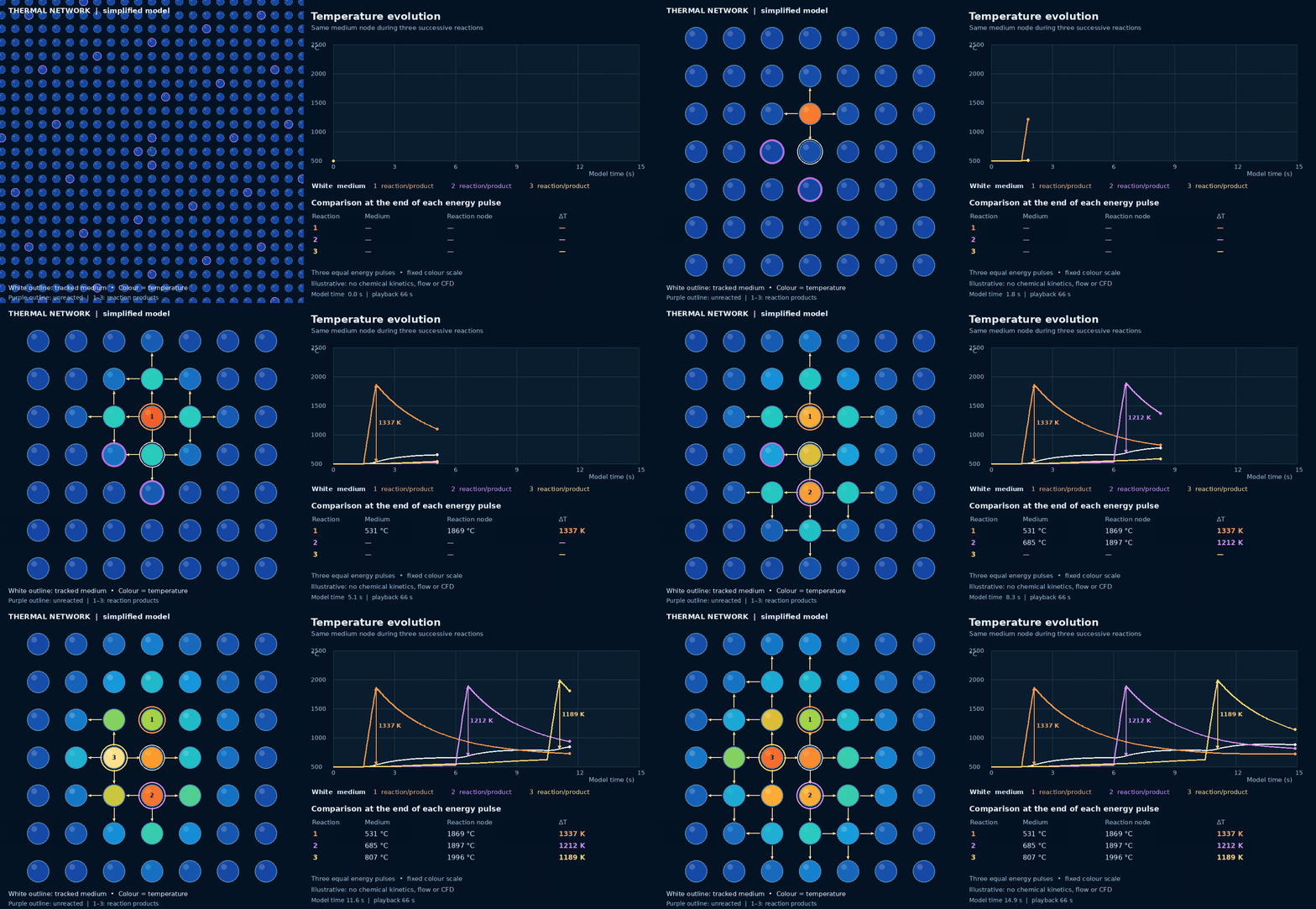
Read the colours and outlines
Colour indicates modelled temperature on a fixed nonlinear scale. A white outline marks the tracked node; purple denotes a node awaiting an imposed pulse, while numbered coloured outlines mark previously heated nodes. Arrows and labels inside the animation are visual conventions, not measured flux vectors or observed chemical products.
Read the time axis
The simulated network spans 15 seconds of model time. The embedded MP4 plays over about 66 seconds. Playback duration is an animation choice, not a real combustor reaction time. Use the player to pause, replay or change playback speed; the GIF is available for download.
Pulse 1 · ΔT1,337 K
Pulse 2 · ΔT1,212 K
Pulse 3 · ΔT1,189 K
These are the testbench’s instantaneous node-to-node temperature differences at a common comparison point at the end of each pulse. Their decrease is specific to the chosen parameters and tracked node. It does not quantify the integrated conduction entropy generation or establish that any real engine’s combustion is more reversible.
| Quantity | Value | Interpretation |
|---|---|---|
| Initial state and capacity | 500 °C; 1 J/K per node | Fixed, illustrative sensible-energy capacity; no species model. |
| Neighbour conductance | 0.12 W/K per link | Prescribed exchange between up to four nearest neighbours. |
| Energy inputs | 3 × 1,500 J; 0.6 s per pulse | Prescribed internal source terms, not calculated chemical rates. |
| Tracked-node temperatures | 500, 624, 766, 811 °C | Reported at approximately 0, 3, 9 and 15 s model time. |
| Summed sensible energy | +4,500 J | Matches the three source pulses in the reported model check. |
| Conduction entropy generated | Approximately 2.08 J/K | Reported for network links only, not for combustion as a whole. |
For node i, the calculated sensible-energy model is:
Node energy balance · fixed thermal capacities
For each connected pair counted once, the model's conduction-related entropy-generation rate is:
Pairwise entropy-generation rate
The temperatures in the entropy calculation are absolute kelvin values. Internal pairwise transfers cancel in the summed energy balance, whereas the prescribed sources increase network sensible energy. In a complete reacting system, this gain would need a corresponding chemical-energy decrease or other explicitly modelled store.
8. From local transport to a cycle benchmark
The proposed External Thermal System (ETS)–Thermodynamic Medium (TM) reading assigns donor-side and receiver-side references to selected, already identified local interactions. These may be neighbouring or overlapping parts of one evolving mixture, not two permanently separate streams. A receiving region may later become a donor. The labels organize a temperature-resolved history; they add no flux, conservation law or independent entropy-production term [1].
A practical research sequence would (1) identify and balance a physical local transfer; (2) locate its two temperatures and cumulative transferred energy without counting reaction heat twice; (3) compare the resulting spatial or time-resolved histories under fixed fuel, inlet, duty, emissions and hardware constraints as appropriate; and (4) recalculate the complete combustor and engine. For Brayton, this includes pressure loss, turbine inlet state and downstream expansion. For Diesel and Otto, it includes the full transient cylinder and mechanical work. The cold-side interaction and remaining cycle processes must also enter an efficiency benchmark.
Only after this model exists can one ask whether a modification to staging, mixing or geometry changes a feasible thermal transport field and the total engine result. Neither parallel-looking T–Q paths nor a reduced isolated conduction term establishes fuel saving, higher net work or a reversible combustion process. A heat-exchanger T–A diagram presumes a physical transfer surface; a comparable “area” coordinate inside an interpenetrating reacting mixture would require its own explicit definition.
9. Fuel temperature and chemical exergy are different questions
Appendix G of the supplied paper separates four quantities that can otherwise be confused: a fuel’s heating value, its chemical exergy relative to a specified environment, the work potential of an actually delivered thermal heat stream, and a complete engine’s net useful work. A nominal reaction-energy difference on a 1 MJ LHV basis is not itself heat transferred through an adiabatic combustor wall.
If a separately specified source truly transfers dQ at a boundary temperature T(Q) to a reversible engine rejecting to T₀, its ideal thermal work potential is:
Conditional thermal-source reference
Here T denotes the local source temperature along the transferred-heat coordinate Q. This conditional expression cannot be applied to fuel chemical energy by merely assigning it an adiabatic flame temperature. The combustion products retain material and potentially chemical exergy; their amount and heat capacity depend on fuel, oxidiser, mixture and equilibrium or kinetic assumptions.
The report’s source-attributed fuel-temperature comparison is exploratory. It does not establish that a higher reported adiabatic flame temperature necessarily gives higher chemical exergy per unit LHV, greater recoverable thermal work or higher engine efficiency. Even for two thermal sources, peak temperature alone cannot order the complete work potential when their T–Q trajectories or transferable heat amounts differ [1].
10. What an engineering validation must establish
The article and animation establish an explanatory bridge. A test of additional engineering value would need to compare an ETS–TM diagnostic against an established reacting-flow and exergy analysis on the same physical case. A useful sequence is:
- Fix the comparison. State the fuel and oxidiser basis, inlet states, geometry, useful output, pressure and emissions constraints, environmental reference and treatment of wall heat transfer. For a reciprocating engine, specify the crank-angle window and moving boundary.
- Resolve the fields. Obtain measured or independently validated computed temperature, composition, reaction-rate, velocity and transport fields. Define grid, averaging interval and sensitivity to any hot-zone classification.
- Close the balances. Reconcile elemental and species flow, formation and sensible enthalpy, chemical conversion, conductive and diffusive face fluxes, advection, pressure losses, work and the complete entropy and exergy budgets. Count each physical mechanism once.
- Test the added diagnostic. Construct candidate ETS–TM temperature–energy histories from attributable fluxes. Compare their explanatory or predictive value with conventional local entropy and exergy maps; a null result is meaningful.
- Recalculate the engine. Only after a feasible change has been defined, compare net shaft work, fuel consumption and the full cycle under the declared constraints. Local conduction loss by itself is not a motor performance rating.
The open Brayton combustor is the most direct first case because it admits a stationary component boundary and continuous throughflow. Diesel and Otto require transient cylinder, injection or flame-front and moving-boundary models. A wall-separated heat exchanger remains a valuable reference for T–Q and T–A reasoning, but its physical transfer area cannot be transplanted unchanged into a mixed reacting gas.
11. Scientific status and sources
Established: reacting-flow energy balances, Fourier conduction, local entropy production and reference-environment exergy accounting. Interpretation of existing theory: comparing defined local interactions with temperature-resolved closed-cycle heat exchange. Proposed CarnotX method: ETS–TM labels and their assembly into a Thermal Matching diagnostic for open combustion. Illustrative: the 100 J two-volume example and A1 network animation. The article offers no independent experimental validation or quantified motor-efficiency improvement.
- CarnotX Research Team, Adiabatic Combustion Chambers and Distributed Local Thermal Transport, Unified Energy B.V., technical position paper v5.36, 11 November 2026. User-supplied source for the analytical framing, two-volume example and A1 model parameters and reported checks. Its ETS–TM application is a proposal; the appended GIF and numerical model are not independent validation.
- Analysis of NO Formation and Entropy Generation in a Reactive Flow, Aerospace 9 (2022), 666. Primary research describing separate conduction, diffusion, reaction and viscous entropy-generation terms in its reacting-flow model; it does not validate ETS–TM.
- NASA Glenn Research Center, Burner Thermodynamics. Educational engineering description of burner mass, fuel and enthalpy accounting and approximately constant pressure; it does not identify combustion with external wall heating.
- Cantera, Adiabatic combustor example. Official modelling example of fuel and air entering an adiabatic reacting control volume; it is not validation of the local example above.
Version 1.2 · 22 November 2026 · CarnotX Academy.
Expanded from the technical position paper, with figures and the A1 animation. System boundaries, model assumptions and scientific status are stated for each level of comparison.